
This article was originally written in Chinese and translated into English by AI.
This is the first article in my Chinese notes for the 2019 edition of CS224N. This lesson explains ways to represent words and how word vectors are calculated.
Stanford’s CS224N in natural-language processing and CS231N in computer vision are two extremely popular artificial-intelligence courses. I originally began studying natural-language processing through the 2017 edition of CS224N and HankCS’s Chinese blog.
NLP has developed rapidly in recent years, and on March 11 Stanford released the lectures from its winter 2019 edition of CS224N. To review the fundamentals myself and make the material more accessible to beginners, I decided to take the latest version again and write a new set of notes.
I recommend reading the corresponding notes on the day after watching each CS224N lecture so that they serve as a review.
Resources
- For the 2017 edition, see the CS224N Study Guide.
- The 2019 material was released on March 11 and did not yet have Chinese subtitles at the time of writing. An English-subtitled version is available on Bilibili.
- Lecture slides, accompanying code, and more official resources

About the Course
Chris Manning remains the course’s resident heartthrob principal instructor. The course focuses on using deep learning for natural-language processing.
Prerequisites:
- Fundamentals of calculus, probability, and linear algebra
- An understanding of machine learning and basic concepts such as gradient descent
- An understanding of deep neural networks
The latest public 2019 edition differs slightly from the 2017 version. Changes include:
- New material on character models, Transformers, multitask learning, and other topics
- PyTorch instead of TensorFlow as the programming framework
1. Ways to Represent Words
Computers store written language through encodings such as UTF-8. They only store and transmit the binary data that represents text. How, then, can a computer understand language?
1.1 WordNet
One traditional natural-language processing method uses WordNet, in which people manually define the various properties of every word.
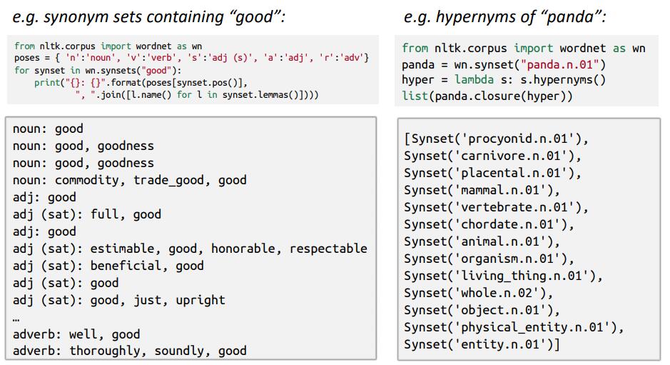
In Chinese, for example, we might define words meaning “good,” “excellent,” and “not bad” as a synonym set expressing high quality. The same word for “good” can join “agree” and “approve” in a synonym set expressing agreement. It can also be synonymous with “very” when expressing degree, as in “so cold.”
Besides synonyms, we can define other properties, such as hierarchical relationships: a panda belongs to the bear family, which belongs to the order of carnivores, which belongs to the class of mammals, and so on.
WordNet nevertheless has clear disadvantages:
- It cannot capture subtle differences between words. We may call “good” and “excellent” synonyms, but they are not identical.
- Words continually acquire new meanings, requiring constant updates.
- WordNet’s definitions are overly subjective.
- Building WordNet requires a great deal of human labor.
- It cannot calculate degrees of similarity between words.
1.2 Discrete Symbols
We can represent every word numerically. In addition to the three methods below, other approaches include n-grams and TF-IDF.
Method one:
Construct a vocabulary that contains, for example, 5,000 common Chinese characters or words, such as [“the,” “I,” “you,” ... “ah”].
Suppose “I” appears in the second position and is represented by 2, while “see” appears in position 703 and is represented by 703. A character absent from the vocabulary is represented by 0. The Chinese sentence meaning “Today I saw a car” can then be represented by the following sequence:
[102, 742, 2, 703, 1842, 12, 3729, 0, 2264]
The sequence is determined by the vocabulary; a different vocabulary produces a different sequence. Given a fixed vocabulary, we can represent a sentence as a sequence of numbers.
Method two: bag of words
We can represent words with one-hot encoding.
Given a vocabulary of length N, one-hot encoding represents every word as a vector of length N. Exactly one position is 1, while every other position is 0.
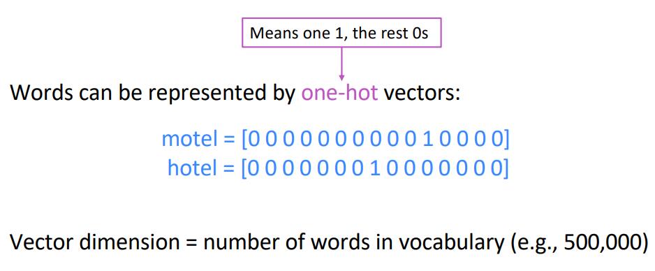
Suppose a vocabulary contains only eight tokens. If “good” is the third token, it can be represented by a vector of length eight:
“good” = [0, 0, 1, 0, 0, 0, 0, 0]
The bag-of-words model ignores word order and grammar. By adding the one-hot encodings of every word in a sentence, we obtain a vector representation of the sentence.
“The articles at 技术杂学铺 are so well written” = [0, 0, 2, 1, 1, 1, 0, 0]
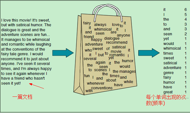
Image from the internet
Because bag of words ignores word order, “I read the article” and “the article reads me” receive the same vector representation even though their meanings are completely different.
Despite this limitation, naive Bayes with bag-of-words features performs well on some text-classification tasks.
Method three: word vectors
As with one-hot encoding, we still represent a word with a vector. The values, however, are no longer limited to integers.
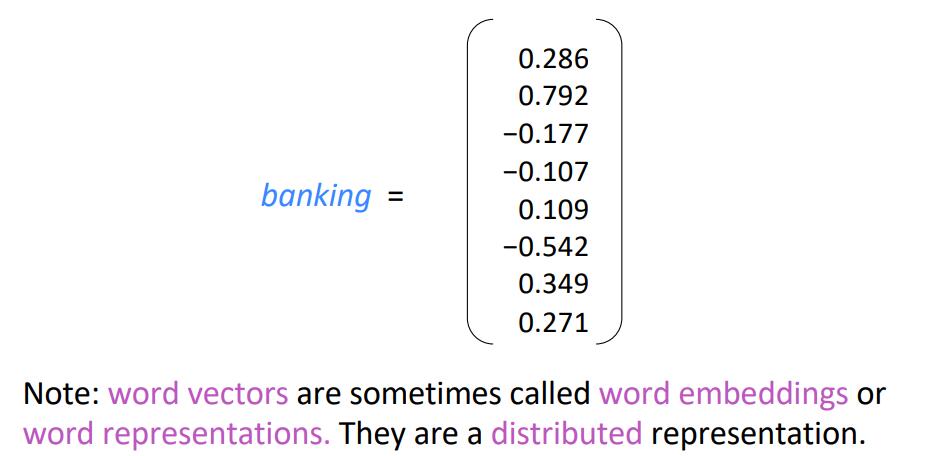
Note: word vectors are also known as word embeddings.
Words with similar meanings have similar word vectors. Similarity may mean that the Euclidean distance between two vectors is small or that the angle between them is small.
We can use the t-SNE dimensionality-reduction algorithm to compress N-dimensional word vectors into two dimensions. Semantically similar words appear close together in the resulting two-dimensional plot: take, get, and make are close, as are were, are, and is.
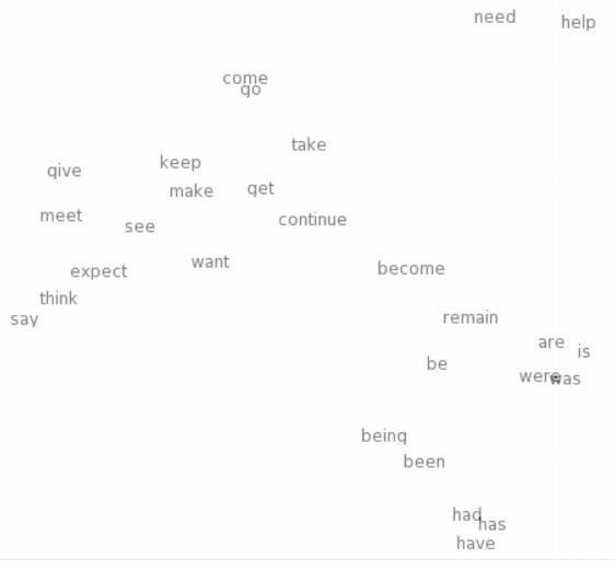
Another interesting property is that although word vectors are merely equal-length sequences of floating-point values, they implicitly encode semantics. The vector for “king” minus the vector for “queen” is approximately equal to “boy” minus “girl.” Similarly, “China” minus “Chinese person” is approximately equal to “Germany” minus “German person.”
Word vectors must be learned with an algorithm. There is currently no single authoritative vector definition for every word: no rule says that “ah” must be [0.1, 0.3, -0.2, ...] or that “good” must be [0.2, -0.1, -0.3, ...]. Open-source vector libraries trained on large text corpora are available on GitHub.
2. Calculating Word Vectors
2.1 Introduction
We assume that a word’s meaning is determined by the words that frequently appear near it. This assumption may seem counterintuitive, but models based on it work remarkably well.
Under this assumption, we can calculate a vector for each word mathematically.
The general idea is:
- Begin with a large amount of text data.
- Represent every word with a fixed-length vector.
- Traverse every word in the text. The current word is the center word, and the n words before and after it form the context.
- Use the similarity between the center and context words to calculate the probability of a context word given the center word, or predict the probability of the center word given its context.
- Continually adjust the word vectors to maximize that probability.
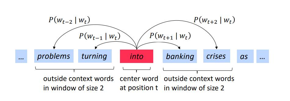
This is the central idea of word2vec: it calculates a vector for every word by predicting the probability of words appearing in text.
The algorithm has many details worth discussing.
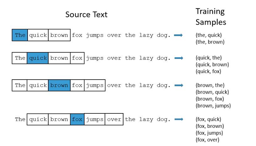
First is context selection. The context of a center word consists of the n words before it and the n words after it. The value of n is set manually.
Consider the tokenized sentence “I today want eat apple , because it is sweet”: [“I”, “today”, “want”, “eat”, “apple”, “,”, “because”, “it”, “is”, “sweet”].
If “apple” is the center word, then when n = 1 its context is [“eat”, “,”]. When n = 2, its context is [“want”, “eat”, “,”, “because”], and so on.
The second detail is word prediction.
Predicting the center word from its context is the continuous bag-of-words model, or CBOW. Predicting the context from the center word is the skip-gram model. Although the two differ slightly, their underlying principle is the same.
Consider predicting the center word from the context.
In “I today want eat apple, because it is sweet,” continue to treat “apple” as the center word and let n = 5. The prediction problem becomes “I want to eat ___ because it is sweet.” We might predict “apple,” “banana,” “chocolate,” or “grape,” but certainly not “house” or “table,” because those words have a very low probability of appearing in a context containing “eat” and “sweet.”
For “I want to eat ____ because it is sweet,” we want the probability of predicting “apple” to be the greatest. Although “banana” and “chocolate” also make semantic sense, the original text says “I want to eat an apple because it is sweet,” so the text is the ground truth.
The corpus will also contain sentences such as “chocolate is sweet” and “I love eating sweet bananas.” After seeing enough examples, the algorithm learns that when “eat” and “sweet” occur in the context, the center word may be “banana” or “chocolate.” “Apple,” “banana,” and “chocolate” therefore acquire similar properties, and their vectors should be close.
Conversely, predicting context from a center word presents “_____ apple _______________” and may predict words such as “sweet” and “eat.”
The ultimate purpose of this word-prediction task is not actually to predict words, but to calculate word vectors. In the task above, foods are more likely to appear near “sweet” and “eat,” so the vectors of words representing foods become similar.
The third detail is the word-prediction algorithm itself: how word2vec adjusts the vectors to maximize the probability of the predicted word. Section 2.2 explains this process.
2.2 Solving for Word Vectors
We use the skip-gram model, which predicts context from a known center word.
2.2.1 Objective Function
Given the word Wt at position t in a sentence, we need to predict the words in its context.
The quality of the predictions can be measured by the following objective function:
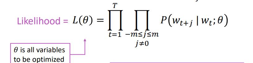
Here, θ represents the parameters to optimize—the word vectors. L(θ) is the product of the probabilities of correctly predicting every context word from every known center word in a passage. A larger L(θ) means better predictions.
Every probability is less than one, however, and multiplying a large number of values below one causes numerical underflow; the final product may become zero. We therefore need to improve the objective.
Taking the logarithm of the expression solves the underflow problem. We generally prefer minimizing an objective to maximizing one, so we also negate the function, turning the original maximization problem into minimization. Finally, we divide by the text length T so that the objective is independent of the amount of text.

A smaller value of the new objective means that the word-prediction task is performing better.
2.2.2 Probability Formula
The probability that o is a context word given the center word c is:
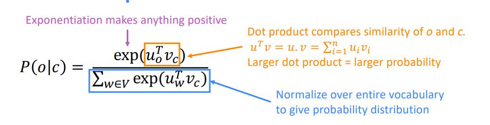
There are two word-vector tables. Their dimensions are vocabulary size N × vector length D; D is set manually and is generally between 100 and 300. V contains center-word vectors, while U contains context-word vectors.
We want P(o|c) to be as large as possible. In other words, the dot product of the center-word vector V for c and the context-word vector U for o should be large.
Readers with a machine-learning foundation will immediately recognize the probability formula as softmax.
We calculate the dot product between the center-word vector V for c and the context-word vector U for every word in the vocabulary. Exponentiation maps the results from (-∞, +∞) to (0, +∞), and normalization then maps them to (0, 1) so that all probabilities sum to one.
Why do we use two vector tables, and why does the largest product determine the prediction? The following provides an intuitive explanation.
Return to “I today want eat apple, because it is sweet.” Given the center word “apple,” we want to predict its context with n = 2. This is a multiclass classification problem whose prediction is one word from the vocabulary.
The training data is:
| Input X | Output Y |
| apple | want |
| apple | eat |
| apple | , |
| apple | because |
One-hot encode the input and output text according to the vocabulary. The problem then becomes training a neural network that receives a word’s one-hot encoding and predicts its context.
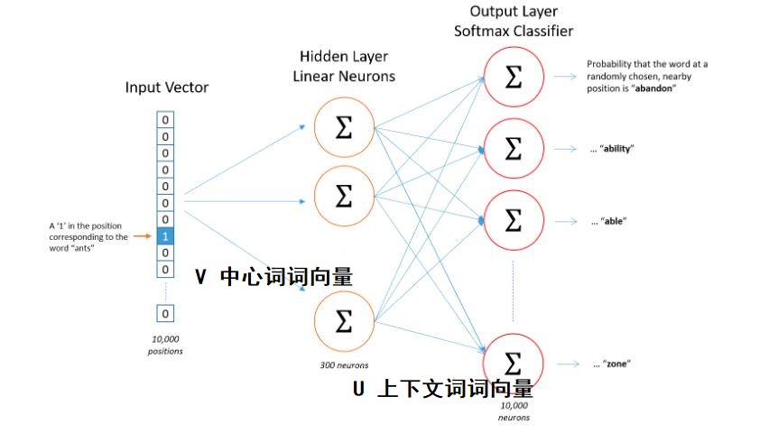
The center-word vector table V contains the weights between the input and hidden layers, while the context-word vector table U contains the weights between the hidden and output layers. Finally, softmax converts the output-layer results into values between zero and one that sum to one.
Once you understand the diagram above, the formula for the probability of context given a center word follows naturally.
Advanced topics: negative sampling can be used to construct training data. Most computation in the model is spent on softmax, so hierarchical softmax can reduce the computational cost.
2.2.3 Solving for the Word Vectors
As the previous section showed, word2vec is essentially a neural network, and both the center-word and context-word vectors are parameters of that network. We can therefore use standard stochastic gradient descent, or SGD, to solve for the parameters.
Initially, the word vectors are randomly initialized. Many initialization methods are possible; parameters may follow a Gaussian distribution N(0, 1), for example.
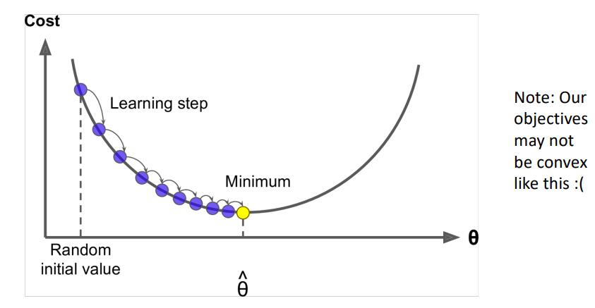
We then use stochastic gradient descent to calculate the gradient of every parameter and update the parameters.
Chris Manning carefully derived the mathematical formulas for gradient descent on the board. I recommend working through the derivation yourself afterward.
We ultimately obtain two word-vector tables, V and U. We can concatenate them. If the center-word vector V for “because” is [0.1, 0.2, 0.3] and its context-word vector U is [-0.4, -0.5, -0.6], the concatenated vector is [0.1, 0.2, 0.3, -0.4, -0.5, -0.6].
A more common—and rather counterintuitive—approach is to add the two tables. The vector for “because” then becomes V + U = [0.1, 0.2, 0.3] + [-0.4, -0.5, -0.6] = [-0.3, -0.3, -0.3].
Experiments show that vectors constructed this way work better, although there is currently no fully satisfying mathematical explanation for why.
Besides calculating word vectors, word2vec can predict user behavior and support recommendation systems. When training word vectors, we provide a sequence of text. When predicting user behavior, we instead provide the user’s sequence of actions. Can you see what to do next? Read this related introduction.
Summary
This lesson explained ways to represent words and how word vectors are calculated.
- Word vectors are now the most common representation of words in natural-language processing. Words with similar meanings generally have nearby vectors.
- Word vectors are trained on large amounts of text. Common algorithms include skip-gram, which predicts context from a center word, and CBOW, which predicts a center word from its context.
- Training word vectors is essentially training a neural network to predict the probability of words appearing. We do not care about the prediction itself, but about the network’s parameters. We use those parameters as word vectors in subsequent NLP tasks.